 Index
Index
- Introduction
- Telescope and CCD parameters
- Throughput
- Atmosphere
- Sky background
- Calculator modes
- Broad-band imaging
- Spectroscopy
- Tunable filter imaging
- Final comments
Introduction
OSIRIS is a versatile instrument and provides many observing modes (see http://www.gtc.iac.es/instruments/osiris/osiris.php), some of which are new or at least non standard. The OSIRIS SNR Calculator is a tool that covers the main observing modes of the instrument. These are: broad-band imaging, medium-band imaging (SHARDs filters), spectroscopy and tunable filter (TF) imaging. This tool estimates signal-to-noise ratios for a given exposure time.
The approach to do that is to compute the expected signal at the detector by taking into account all the elements involved in the detection process (telescope, lenses, filters, detectors, etc.) as well as the external factors contributing mainly to photon losses or noise (atmosphere, sky brightness, Moon brightness). Many of the factors are well known or may be measured accurately, for instance the instrument efficiencies, while others must be estimated or assumed (e.g. sky brightness).
The OSIRIS Signal-to-noise Calculator has been developed by the author as a Java program to be executed through a web navigator. At present it can be accessed at https://gtc-phase2.gtc.iac.es/science/OsirisETC/html/Calculators.html. To run the application Java JRE 1.6 or later should be installed on the client machine. Also, the JNLP MIME type should be set to application/x-java-jnlp-file to be opened by javaws on the client navigator.
As the GTC/OSIRIS commissioning is progressing, real behaviour and most recent efficiencies are incorporated into the calculator. Also, not all the subsystems are available yet: blue TF and blue order-sorter filters. All (except the blue TF) are implemented in the calculator but this DOES NOT IMPLY THAT THEY ARE WORKING AT THE TELESCOPE. Visit the GTC OSIRIS page to check what is available and what is not.
Telescope and CCD parameters
The collecting area of the GTC is taken to be 741,400 cm2. The CCD pixel size has been measured during commissioning and it is 0.12718 arcsec.
Although it is possible to define CCD binning of 1x1, 2x2, 1x2, and 2x1, only binning 2x2 only binning 2x2 is defined as standard in all observing modes. There are three readout modes: Spectroscopy, Imaging and Acquisition, but the last one it is not suitable for scientific applications, in general.
The CCD characteristics used in the calculators are listed in the next table and correspond to commissioning values:
Mesurements of dark current indicate a mean dark noise of 1.8 e-/hour/pixel.
| Readout mode | Imaging | Spectroscopy | Acquisition |
| Readout velocity (kHz) | 200 | 100 | 500 |
| Gain (e-/ADU) | 0.95 | 1.18 | 1.46 |
| Binning | 2x2 | 2x2 | 2x2 |
| Readout time (s) | 24.0 | 42 | 7.8 |
| Readout noise (e-) | 4.5 | 3.5 | 8 |
Preliminary measurements of dark current after changing to the new cryostat (February 2010; Antonio Cabrera private communication) indicate a mean dark noise of 1.8 e-/hour/pixel.
Throughput
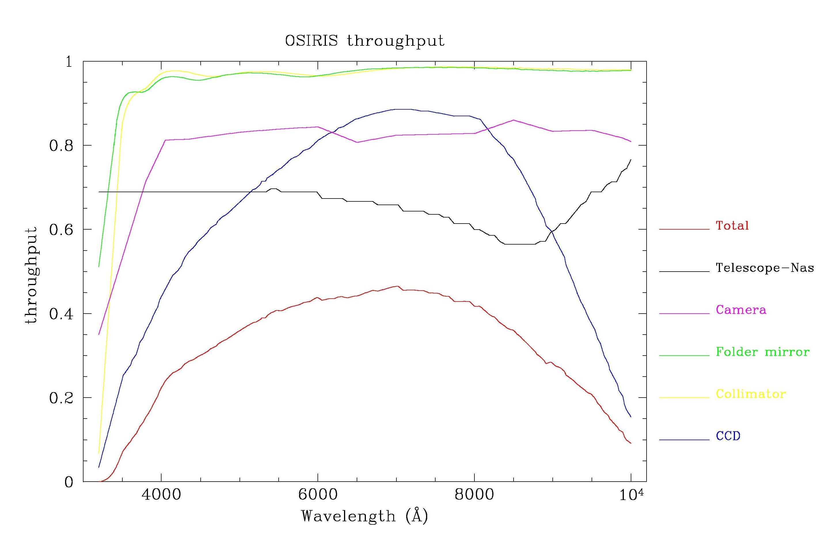
Before OSIRIS was mounted at the telescope, most of the transmissions and efficiencies of the optical subsystems and CCDs were measured in laboratory conditions. Broad-band and order sorter filters transmissions have been obtained during commissioning, as well as for the available grisms. TF transmission has been measured at some spectral ranges and has been updated (~80% lower that theoretical).
The throughput of the instrument (without filters or grisms) is plotted in the following figure:
Atmosphere
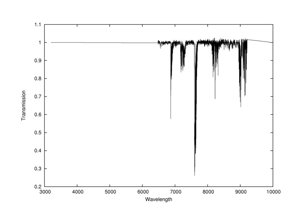
The simulator computes atmospheric extinction and absorption. Atmospheric extinction at each wavelength is obtained from standard curves measured at the observatory, which are given in magnitudes per airmass. Atmospheric transmission is also taken into account using the following curve:
Sky background
Nigh sky emission is also taken into account both in TF imaging and in spectroscopy. The spectrum used is from (Hanuschik, R.W. , 2003, A&A, 407, 1157) which is a high-resolution flux-calibrated spectrum from
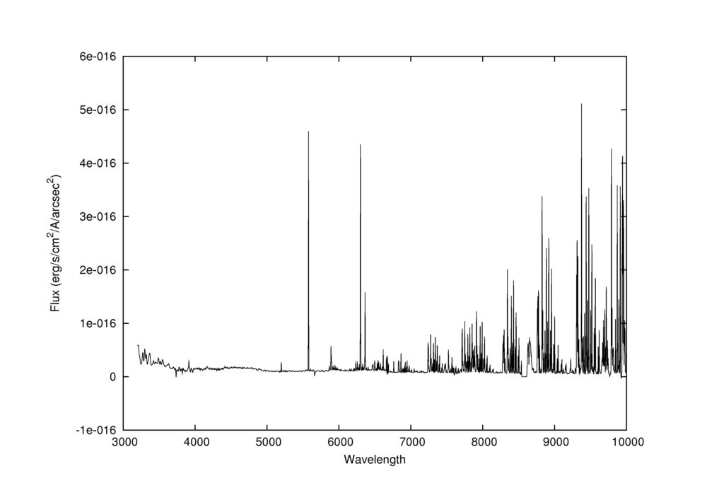
For TF imaging, spectroscopy, and imaging using order sorter or user-defined filters, the sky background is computed from that spectrum. In broad-band mode using the standard ugriz filters, sky background is assumed to be the mean at the observatory.
To take into account moonlight we have classified nights into three types: dark, grey, and bright. For all modes, the surface brightness of the sky background is increased by an amount depending on the type of the night and on the spectral range. These are listed in the next table:
|
|
U |
B |
V |
R |
I |
Z |
|
Range(?) |
3400-4000 |
4000-4950 |
4950-5950 |
5950-7150 |
7150-8700 |
8700-10000 |
|
Grey |
2.1 |
1.1 |
0.4 |
0.3 |
0.2 |
0.2 |
|
Bright |
5.0 |
3.2 |
1.8 |
1.0 |
0.7 |
0.7 |
This approach is the same as that used in the ESO ETC calculators.
Take into account that sky brightness vary from night to night and even during one night. Also, Moon contribution is strongly depending on the angular distance from target to Moon and on airmass. Therefore, these are the main factors affecting estimations of signal-to-noise.
Calculator modes
We describe here and in the following sections the operation of the OSIRIS Calculator.
For all modes, user must choose:
- Focal station (Nasmyth or Cassegrain)
- CCD readout mode
- Binning
- Type of source (point-like or extended)
- Airmass
- Seeing FWHM (arcsec)
- Moon (bright, grey or dark)
- Fraction of flux (if source type is point-like) in %
- Number of exposures
- Exposure time for a single exposure (s)
Fraction of flux refers to the percentage of the total flux of the source to be considered for SNR calculations. Here a Gaussian point spread function is assumed for point sources. It is related to the radius of the aperture as,

where FWHM is the seeing and EF is the fraction of flux.
For extended sources this parameter is irrelevant.
Time to saturation is also computed assuming that the maximum counts per pixel is 50,000. For point-like sources it is assumed that source is centred at one pixel, therefore, the saturation time computed is an upper limit.
When the tool starts, a window with three independent tabs is open. Each tab corresponds to an observing mode. All parameters are initialized at a default value, so check all parameters to meet your requirements. By clicking on 'Compute' the calculations are done and the output is shown at the right panel. If some error or warning exists, a red message will appear below that button. If all is OK, the message will be '...done'. You can change from panel to panel as many times as you need, but take into account that parameters ARE NOT TRANSFERRED between them.
The tool can be stopped by clicking 'Quit' at any of the panels. It is possible to send the output to a printer by clicking button 'Print'. For the spectroscopic mode there are two queries to the printer: one for the text output panel and the other for the SNR/pixel plot.
The output is different from mode to mode, but there is some information that is common to all modes:
- Focal station
- Type of source
- Readout mode and ADU
- Moon
- Binning
- Encircled energy or fraction of flux
- Band information
- Total exposure time and total time (i.e. including readouts ONLY)
Broad-band imaging
The default readout mode is Imaging with a readout speed of 200 kHz. There are three options for this observing mode:
- Broad-band imaging with the standard filters u'g'r'i'z'.
- Intermediate-band imaging with the order sorter filters.
- User-provided filter. In this mode the user should specify filter characteristcs: central wavelength, width, and transmission.
In case (1) the input target magnitude corresponds to the selected filter. In cases (2) and (3) AB magnitudes are used. In all cases, target magnitude is assumed to be constant trough the filter bandwidth.
Output:
- It includes the total efficieny of the system and the area (in pixels) of the source over the detector, that is, the area where computations are made.
- If the source is extended, computations are made in one pixel.
- Next is the counts from source, count from sky, counts/pixel from sky, noise from source, noise from sky, total noise, signal-to-noise, and time for saturation for a single exposure.
- If source or sky saturate in a single exposure a message will appear.
- For the total exposure, the output includes total on-source time and total time (i.e. including readouts).
- The total readout noise, total noise and final signal-to-noise ratio are also shown.
- If source is extended, calculations per arcsec**2 are also shown.
Spectroscopy
The default readout mode is Spectroscopy with a readout speed of 100kHz. User should select a grims from the list. Characteristics of grims are listed in the following table:
|
Grism |
lc (Å) |
Spectral
range (Å) |
Dispersion (Å/mm) |
Dispersion (Å/pixel) |
Resolution (dl) with slit =0.6” |
Peak
eff. |
|
R300B |
4560 |
3600
– 7000 |
188.7 |
2.48 |
11.9 |
0.64 |
|
R300R |
6865 |
4800
– 10000 |
282.7 |
3.87 |
18.57 |
0.42 |
|
R500B |
4830 |
3440
– 7600 |
130.7 |
1.77 |
8.49 |
0.53 |
|
R500R |
7310 |
4800
– 10000 |
171.3 |
2.44 |
11.71 |
0.36 |
|
R1000B |
5510 |
3630
– 7500 |
76.7 |
1.06 |
5.09 |
0.54 |
|
R1000R |
7510 |
5100
– 10000 |
92.7 |
1.31 |
6.29 |
0.41 |
|
R2000B |
4780 |
3950
– 5700 |
31.4 |
0.43 |
2.06 |
0.66 |
|
R2500U |
4025 |
3440
– 4610 |
22.1 |
0.31 |
1.49 |
0.81 |
|
R2500V |
5210 |
4500
– 6000 |
28.7 |
0.40 |
1.92 |
0.76 |
|
R2500R |
6590 |
5575
– 7685 |
36.4 |
0.52 |
2.49 |
0.53 |
|
R2500I |
8740 |
7330
– 10000 |
47.9 |
0.68 |
3.26 |
0.35 |
The efficiency curves used for all the grisms are those measured with real calibration stars and updated - July 2011.
- 1x1 standard pixel size
- 1x2 binning along dispersion
- 2x1 binning along spatial direction (slit)
- 2x2 binning along both directions
The size along the slit, given in units of the seeing, determines the number of pixels along the slit to compute signal from source, sky background, readout noise and dark current. For point sources, seeing profile is assumed to be Gaussian. For extended sources this parameter does not apply and computations are made per pixel along slit. In this mode there are two options:
- Target is a pure continuum source. In this case, the spectrum is assumed to be of constant magnitude trough the spectral range of the grism and magnitude is in the AB system.
- Target is a continuum + emission line source. For the continuum, assumptions are the same as in case (1). For the emission line, user can define the central wavelength, FWHM and total intensity of the line (erg/s/cm**2). A Gaussian profile is assumed for the emission line.
Output:
- There are two output panels.
- Central panel is a plot of the signal-to-noise ratio per pixel along spectral direction.
- The right panel includes information about grism, pixel size, effective resolution, fraction of total flux that enters the slit (if the source is point-like), and total exposure and observing times.
- For extended sources the plot corresponds to one pixel along slit.
- Note that noise depends on the sky background, therefore in the SNR plot sky emission and absortion features will appear.
Tunable Filter imaging
The default readout mode is Imaging with a readout speed of 200 kHz.
First, the TF should be selected. At this moment (February 2010) blue TF is not available so that a message will show up if this is selected. Desired TF wavelength and FWHM should be selected. The tool checks the possible FWHMs for the given wavelength and chooses the nearest one. Then, the order sorter filter is selected automatically from the list of available filters. If no filter exists, a message will appear below the 'Calculate' button. Use the TF Setup Tool to obtain the possible values of the FWHM for a given wavelength.
As in spectroscopy, user has two options:
- Target is a pure continuum source. In this case, the spectrum is assumed to be of constant magnitude trough the spectral range of the TF+order sorter filter and magnitude is in the AB system.
- Target is a continuum + emission line source. For the continuum, assumptions are the same as in case (1). For the emission line, user can define the central wavelength, FWHM and total intensity of the line (erg/s/cm**2). A Gaussian profile is assumed for the emission line.
Output:
- User should look carefully at the output window to check that central wavelength and FWHM of the TF meet his/her requirements. Some information related to the TF is shown in the output panel. The Free Spectral Range (FSR) is the size of the spectral range (centred at the tunned wavelength) where only one interference order is transmitted through the etalon. Note that no order sorter filter will be selected if theFSR is smaller than the width of any of the filters available, and then, no calculations will be made.
- Total efficiency of the system at the selected wavelength is shown.
- The combined effect of atmosphere extincion and absorption is computed and shown (in %), i.e. a high value means a high extinction and absorption. Check this number and use the TF Setup Tool to select a wavelength free of strong telluric lines.
- If a strong sky emission line is +/- 5 Å from the central wavelength, a message will appear, showing the wavelength of this line. Check that and use the TF Setup Tool to select a wavelength free of strong sky emission lines.
In this mode, signal-to-noise ratios are separated in continuum, line and total.
- Continuum SNR takes into account the continuum of the source as the signal only, and the noise is computed from the source, sky background and detector noise.
- Line SNR takes into account the emission line as the signal only, and the noise is computed from the source emission line, source continuum, sky background and detector noise.
- Total SNR takes into account both continuum and emission line as the signal.
The remaining of the output is similar to that of the Broad-Band mode.
Final Comments
The author (J. Ignacio Gonz?lez-Serrano) is the only responsible for this tool. An effort has been made to make a realistic simulation of the OSIRIS instrument although some effects are very difficult (or even impossible) to predict accurately.
Please contact the author
for comments, suggestions, complaints, and
errors or inconsistencies found; they are all welcome.
Last modified: 27 May 2013
38712 - Breña Baja - La Palma, España
Tel?fono: +34 922 425 720 | Fax: +34 922 425 725
e-mail: gtc [at] gtc.iac.es


